
working through a maze part 2
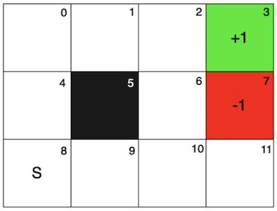
This time the grid is a bit different, but is also quite the same. The goal state now gives a +1 reward, while the danger cell gives -1. There is still a blocked cell (5) and now all runs start from the initial state 8.
The purpose of this exploration is to test the differences in performance between On/Off Policy MC control methods vs. On/Off Policy TD control methods (SARSA and Q-learning).
- On-policy MC control is implemented using first-visit methods.
- Off-policy MC control initializes the arbitrary “b” policy as one that gives an equal amount of probability to each action from a given state. It uses the every-visit method.
- On-policy TD control and Off-policy TD control follow the given SARSA and Q-learning definitions respectively.
Hyper Parameters
For MC control there are two hyper parameters: epsilon and gamma. For TD control there are three hyper parameters: alpha, epsilon and gamma.
pythonimport itertools

param_grid = {
    'epsilon': [0.01, 0.1, 0.3],
    'gamma': [0.9, 0.99, 0.9999],
    'alpha': [0.01, 0.1, 0.5],
}

# Create a list of all hyperparameter combinations
all_params = list(itertools.product(*param_grid.values()))

# Iterate through each combination for a different number of episodes
for num_episodes in [10, 50, 100]:
    success_rates = []
    for params in all_params:
        epsilon = params[0]
        gamma = params[1]
        alpha = params[2]

        # Create instances of GridWorld for each algorithm
        gw_test = GridWorld(height=3, width=4, goal=3, goal_value=1, danger=[7], danger_value=-1, blocked=[5])

        success = 0
        num_of_tests = 100

        for x in range(100):
            gw_test.reset_training()

            # on_policy_mc_control(gw_on_mc, num_episodes=num_episodes, epsilon=epsilon, gamma=gamma)
            # off_policy_mc_control(gw_off_mc, num_episodes=num_episodes, epsilon=epsilon, gamma=gamma)
            on_policy_td_control(gw_test, num_episodes=num_episodes, alpha=alpha, epsilon=epsilon, gamma=gamma)
            # off_policy_td_control(gw_off_td, num_episodes=num_episodes, alpha=alpha, epsilon=epsilon, gamma=gamma)

            if evaluate_policy(gw_test): success += 1

        success_rates.append(success / num_of_tests)

    sorted_rate_indexes = sorted(range(len(success_rates)), key=lambda i: success_rates[i])
    best_rates = [success_rates[i] for i in reversed(sorted_rate_indexes)]
    best_params = [all_params[i] for i in reversed(sorted_rate_indexes)]
I wrote a small bit of code to do a parameter search over a small space. I knew that I wanted the discount factor to be 0.9-0.9999 since long-term planning was preferred to find a continuous path to the goal state even if it was a longer one. For exploration, since there aren’t a lot of possible states, I knew that the rate should be small, so 0.01, 0.1 and 0.3. For alpha, I tried values of 0.01, 0.1 and 0.5 and did not go higher to not introduce too much instability into the TD method and overshoot the state-action values. I also did the search only over a small number of episodes (10, 50, 100 and maybe 150, 200 if necessary) because I wanted to prioritize hyper parameters that made each method converge to a high success rate as fast as possible. Above 100 episodes, any hyper parameters gave a decent result and it made it harder to decide. Plus computationally it was a lot harder to search the space with a high number of episodes.
The code iterated over all possible combinations of the hyper parameters for the respective method and returned back the best parameters. A lot of the hyper parameters returned the same results and some were very varied in results, so in that case I used my best intuition to pick the parameters.
- On-policy MC control: epsilon = 0.3, gamma = 0.9999
- Off-policy MC control: epsilon = 0.3 , gamma = 0.9999
- On-policy TD control: alpha = 0.1, epsilon = 0.3 , gamma = 0.9999
- Off-policy TD control: alpha = 0.1, epsilon = 0.3 , gamma = 0.9999
Findings
There are two areas of comparison that I noticed between the methods. The first was the speed at which training occurred.
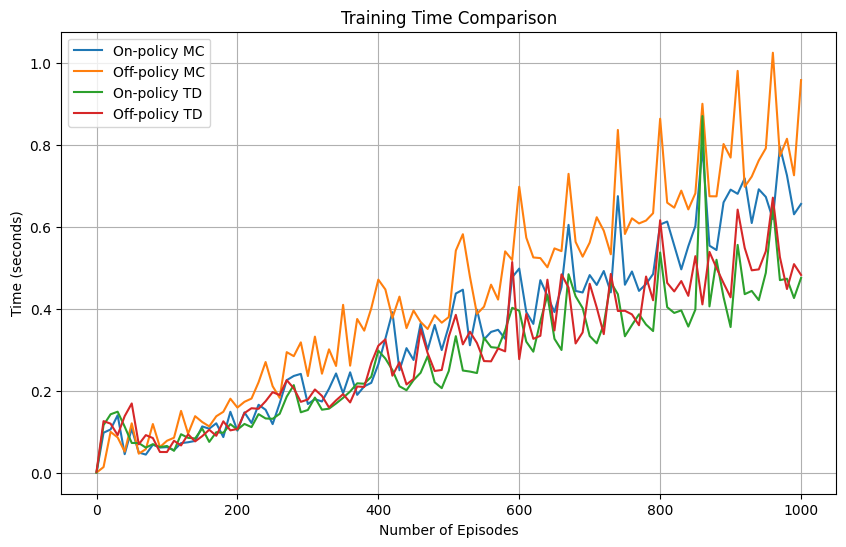
From the figure we can see that the MC control methods had on average a higher training time than the TD methods. As we approach larger numbers in terms of the number of episodes used in training, we can see that the differences are more evident and it is probably the case that as the number of episodes increases these differences will only get more significant. Off-policy MC seems to also be slightly faster than On-policy MC and this is most likely caused by the fact that in On-policy MC I used the first-visit method, which introduces an extra for loop to check all previous state-action pairs for matches.
The second area of comparison is in the success rate of the policy generated by each method after different amounts of training. This can show the sample efficiency of the method, or how well it can find an optimal policy using a small number of examples. I tested this by generating a policy using each method 50 times at 0,10,20,...,1000 episodes and seeing if the generated policy could get to the goal state from the initial state. I then got a percentage out of 50 and plotted it as seen below for each method. This took me approximately 1 hour and 45 minutes to complete. If I had stronger hardware and the knowhow of how to parallelize this without dealing with race conditions on shared data, I would have tried going to higher episode number counts.
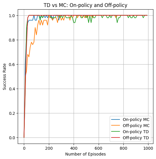
From the graph we can see that the TD methods are the fastest to reach high success rates, with the smallest number of episodes trained on.
Out of the MC methods, off-policy MC seems to perform worse than on-policy MC, but as we saw in the previous figure, it does train faster. I think the data here is a bit misleading though and on-policy MC is just very good at this specific problem. This is because even at 1000 episodes if I run the on-policy MC control algorithm it sometimes gives me incorrect policies for state 11. This is not reflected in these graphs because the agent does not need to visit state 11 in order to finish the grid. Maybe in larger and more complicated graphs the result of this test would be much different.
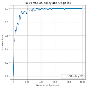
Both on and off policy TD had incredibly good convergence for a small amount of episodes, but there is a major difference. On-policy TD can be seen to have dips in its success rate even at very high number of episodes compared to off-policy TD which reaches 100% success rate and stays there the entire time. This is caused by the different ways that the algorithms do value updates to the state-action values. On-policy generates a new policy at the beginning of each episode and follows it throughout the episode to update values. Off-policy follows argmax of the next state’s possible actions and provides a more up to date action based on the current information gained from the episode. This can mean that the off-policy method explores differently and is maybe more likely to not get trapped in local minima unlike its on-policy counterpart. It is likely that as the number of episodes increases past 1000 that on-policy TD would also stabilize at 100% success rate.
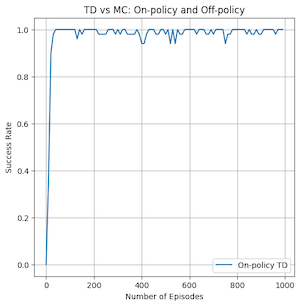
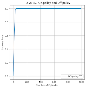
In conclusion, it is clear to see that off-policy TD performed the best out of all the methods. It had fast training times, the quickest convergence and the most stable results.
Code
python"""ON-POLICY MC CONTROL"""

def on_policy_mc_control(gw, num_episodes=1000, epsilon=0.1, gamma=0.9):
    for _ in range(num_episodes):
        episode = gw.generate_episode()
        G = 0
        for t in reversed(range(0, len(episode))): # go backwards through episode
            state, action, reward = episode[t]
            G = gamma*G + reward

            # check if the state-action pair appears earlier
            earlier = False
            for i in range(0, t):
                s, a, r = episode[i]
                if s == state and a == action:
                    earlier = True
                    break

            if not earlier:
                gw._returns[state][action].append(G)
                gw._Q[state][action] = np.mean(gw._returns[state][action])

                # generate e-greedy policy
                A_star = max(gw.get_actions(state), key=gw._Q[state].get)

                num_of_actions = len(gw.get_actions(state))
                for a in gw.get_actions(state):
                    if a == A_star:
                        gw._policy[state][a] = 1 - epsilon + epsilon/num_of_actions
                    else:
                        gw._policy[state][a] = epsilon/num_of_actions

"""OFF-POLICY MC CONTROL"""

def off_policy_mc_control(gw, num_episodes=1000, epsilon=0.1, gamma=0.9):
    C = {}
    policy_b = {} # arbitrary soft policy
    for s in gw.get_states():
        C[s] = {Action(a): 0.0 for a in range(4)}

        # initialize policy as equal probability for each action
        policy_b[s] = {Action(a): 0.0 for a in range(4)}
        valid_actions = gw.get_actions(s)
        for a in valid_actions:
            policy_b[s][a] = 1/len(valid_actions)

    # start algorithm
    for _ in range(num_episodes):
        episode = gw.generate_episode(policy=policy_b)
        G = 0.0
        W = 1.0

        for t in reversed(range(0, len(episode))): # go backwards through episode
            state, action, reward = episode[t]
            G = gamma*G + reward

            C[state][action] += W
            gw._Q[state][action] += (W/C[state][action]) * (G - gw._Q[state][action])

            # generate argmax policy for state
            A_star = max(gw.get_actions(state), key=gw._Q[state].get)
            for a in gw.get_actions(state):
                if a == A_star:
                    gw._policy[state][a] = 1
                else:
                    gw._policy[state][a] = 0

            # if A_t != policy(S_t) break
            if action != A_star:
                break

            W *= 1/policy_b[state][A_star]

"""ON-POLICY TD CONTROL"""

def on_policy_td_control(gw, num_episodes=1000, alpha=0.1, epsilon=0.1, gamma=0.9):
    # make sure all Q(terminal, -) = 0, since all values can be arbitrary, just set all to 0
    gw.reset_training()

    for _ in range(num_episodes):
        gw.generate_policy(epsilon)

        state = 8
        counter = 0
        possible_actions = gw.get_actions(state)

        # choose A from S using policy derived from Q
        action = np.random.choice(possible_actions, p=[gw._policy[state][a] for a in possible_actions])

        while True:
            next_state = gw._state_from_action(state, action)
            reward = gw.get_reward(next_state)

            # if state is terminal or episode is over 30, terminate
            if gw.is_terminal(next_state) or counter >= 30:
                # if next state is terminal then gamma * Q(S', A') = 0
                gw._Q[state][action] = gw._Q[state][action] + alpha * (reward - gw._Q[state][action])
                break

            possible_actions = gw.get_actions(next_state)
            # choose A' from S' using policy derived from Q
            greedy_action = np.random.choice(possible_actions, p=[gw._policy[next_state][a] for a in possible_actions])

            gw._Q[state][action] += alpha*(reward + gamma*gw._Q[next_state][greedy_action] - gw._Q[state][action])

            # update values
            state = next_state
            action = greedy_action
            counter += 1

    # generate deterministic policy at the end of training
    gw.generate_policy(epsilon)


"""OFF-POLICY TD CONTROL"""

def off_policy_td_control(gw, num_episodes=1000, alpha=0.1, epsilon=0.1, gamma=0.9):
    # make sure all Q(terminal, -) = 0, since all values can be arbitrary, just set all to 0
    gw.reset_training()

    for _ in range(num_episodes):
        # generate e-greedy policy from Q
        gw.generate_policy(epsilon)

        state = 8
        counter = 0

        while True:
            possible_actions = gw.get_actions(state)
            # choose A from S using e-greedy policy derived from Q
            action = np.random.choice(possible_actions, p=[gw._policy[state][a] for a in possible_actions])

            next_state = gw._state_from_action(state, action)
            reward = gw.get_reward(next_state)

            # if state is terminal or episode is over 30, terminate
            if gw.is_terminal(next_state) or counter >= 30:
                # if next state is terminal then gamma * Q(S', A') = 0
                gw._Q[state][action] = gw._Q[state][action] + alpha * (reward - gw._Q[state][action])
                break

            # get max_a for max_a Q(S', a) in update
            A_star = max(gw.get_actions(next_state), key=gw._Q[next_state].get)

            gw._Q[state][action] += alpha*(reward + gamma*gw._Q[next_state][A_star] - gw._Q[state][action])

            state = next_state
            counter += 1

    gw.generate_policy(epsilon)