
working through a maze
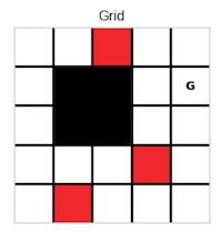
The Gridworld consists of a grid of cells, each representing a distinct state in which an agent can operate. The agent has four possible actions available to it: moving north, south, east, or west. For every state within the grid, the agent selects one of these actions with an equal probability of ¼. Once an action is chosen, the agent moves in the specified direction with certainty (probability of 1). If the agent attempts to move into a wall, goes off the grid, or lands on a blocked cell (designated as black cells), it is unable to proceed and receives a reward of 0. Similarly, if the agent moves to any other cell within the grid that is not associated with a specific event, it also receives a reward of 0.If the agent reaches a red cell (representing fire), the game terminates immediately, and the agent incurs a penalty of -5. Conversely, if the agent successfully navigates to the goal cell (marked as G), it receives a reward of +5, at which point the game also concludes.
The point of this excersize was to implement basic a markov decision process by solving the linear system for the values of each state and dynammic programming through a value iteration algorithm. The code implements the algorithms and this blog shares the results of the implementations.
1. Linear Solver
pythondef solve_linear_system(self, discount_factor=1.0):
    """
    Solve the gridworld using a system of linear equations.
    :param discount_factor: The discount factor for future rewards.
    """

    # find v(s) for every s

    A = np.array(np.zeros((self._width*self._height, self._width*self._height)))
    b = []

    for s in range(0, self._width*self._height):

        b_value = [0]

        if self.is_terminal(s) or s in self._blocked_cells:
            # terminal or blocked cells value is determined solely by their own value (= reward)
            A[s][s] = 1
            b_value[0] = self.get_reward(s)
        else:
            """
            the idea here to construct A is the following:
            ex. state = 0 and assuming noise = 0 for simplicity.
            since immediate reward for each state is 0,
            v(0) = 1/4*γ*v(0) + 1/4*γ*v(0) + 1/4*γ*v(1) + 1/4*γ*v(5)
            (1 - 1/2*γ)v(0) - 1/4*γ*v(1) - 1/4*γ*v(5) = 0
            We can see that if the state takes an action that brings it back
            to itself, we subtract that probability*gamma from 1. If it goes to
            another state, we have -1*probability*gamma coefficient for the value
            of that next state. We use this knowledge to build A now.
            """
            A[s][s] = 1 # initialize the coefficient of the state itself as 1

            num_of_actions = len(self.get_actions(s))
            action_probability = 1/num_of_actions

            for a in self.get_actions(s):

                # include transition probabilities that incorporate noise
                transitions = self.get_transitions(s, a)
                # probablistic outcome of action selection simply adds transition probability as coefficient factor
                for transition in transitions:
                    next_state = transition["state"]
                    state_prob = transition["probability"]

                    if next_state == s:
                        # same state so subtract
                        A[s][s] -= action_probability * state_prob * discount_factor
                    else:
                        # add coefficient to correct place in A
                        A[s][next_state] += -1 * action_probability * state_prob * discount_factor
        b.append(b_value)

    b = np.array(b)

    values_grid = np.linalg.solve(A, b)

    # convert the numpy array to a list and set it to grid values
    for i in range(0, len(values_grid)):
        self._grid_values[i] = values_grid[i][0]
We first try the MDP algorithm with a discount factor of 0.95
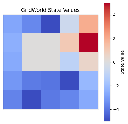
We can see that the linear solver does not result in the optimal policy. The figure on the left we can see a visualization of the value of each state. The state (1, 0) represents a local maximum, where the states on the left side of the grid will end moving towards it instead of the goal state. The goal state (1, 4) is the other maximum, and the states on the right side of the grid will end up in that goal state following this policy.
Then with a discount factor of 0.75
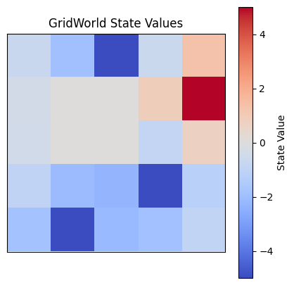
We can see that for a discount value of 0.75, the linear solver finds the values of states to be slightly smaller (signified by colours being lighter), but the values are proportionally the same. By this, I mean other than the goal and danger states which have a set values of 5 and -5 respectively, the other states have the same values as the first solution in terms of relation to the values next to them. This results in the same policy being deduced.
2. Value Iteration DP Algorithm
pythondef value_iteration(gw, discount, tolerance=0.1, plot_delta=True):
    delta = 0
    delta_values = []
    gw.solve_linear_system(discount)

    # loop until delta < threshold
    while True:
        delta = 0
        gw.create_next_values()
        for s in gw.get_states():
            v = gw._grid_values[s] # v <- V(s)

            # V(s) -> max_a sum_{s', r} p(s',r|s,a)[r + gamma * V(s')]
            max_a = float("-inf")
            num_of_actions = len(gw.get_actions(s))
            for a in gw.get_actions(s):
                transitions = gw.get_transitions(s, a)
                value = 0
                for transition in transitions:
                    # p(s',r|s,a)[r + gamma * V(s')] for s'
                    value += transition["probability"] * discount * gw._grid_values[transition["state"]]
                max_a = max(max_a, value)

            gw.set_value(s, max_a)

            # delta <- max(delta, |v - V(s)|)
            difference = abs(v - max_a)
            delta = max(delta, difference)

        # collect the max delta value
        delta_values.append(delta)

        gw.set_next_values()

        if delta < tolerance:
            break

    # output a deterministic policy
    gw.create_next_values()
    for s in gw.get_states():
        max_a = float("-inf")
        argmax = -1
        for a in gw.get_actions(s):
            transitions = gw.get_transitions(s, a)

            # sum_{s', r} p(s',r|s,a)[r + gamma * V(s')]
            value = 0
            for transition in transitions:
                value += transition["probability"] * discount * gw._grid_values[transition["state"]]

            # calculate argmax of actions
            if value > max_a:
                argmax = a
                max_a = value
        gw.set_value(s, argmax)
    gw.set_next_values() # set the policy to be the _grid_values
I use a while loop to iterate over every state which is not blocked, a danger or a goal state. For each I save their current value and use another loop to iterate over the possible actions. For each action I use the get_transitions function to get the next states and respective probabilities. I multiply "transition_probability * discount * V(next_state)" for each possible next state and then add these values together to get the new value for the state. I then compare this value to the state’s original value and keep track of which state has the biggest difference between the two. If the largest difference is bigger than 0.1, the while loop is broken. From here, for each state the value of the state is calculated again but this time the action resulting in the biggest value is saved and used as the action in the deterministic policy.
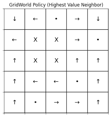
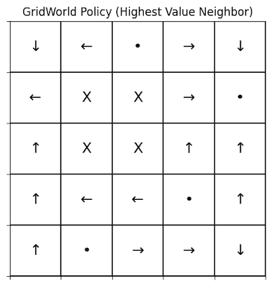
i) with transition noise = 0.0
In the first figure we see the policy that was deduced by the value iteration, where the numbers are the integer representation of an action, with the exception of -5.00, which represents the value of the danger cell. We can see in the second figure, where the values are converted to arrows, that starting from each state you can follow a continuous path to the goal state. This means we have found an optimal policy!
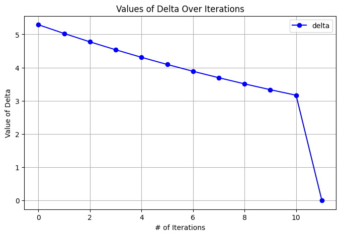
We can also see how the delta converges over the 11 total iterations. It slowly gets lower and lower before dropping completely to 0 on the last iteration. This is because the transition function is deterministic and as all values slowly converge, the values of other states are based on stationary values. This leads to the last difference being about 3 which is the difference between the last state and its actual value and then drops off to 0 as that state is determined by the stationary values around it.
Since the policy has great quality (every state can reach the goal state) and the delta converged quickly, I believe the algorithm was very effective in this case.
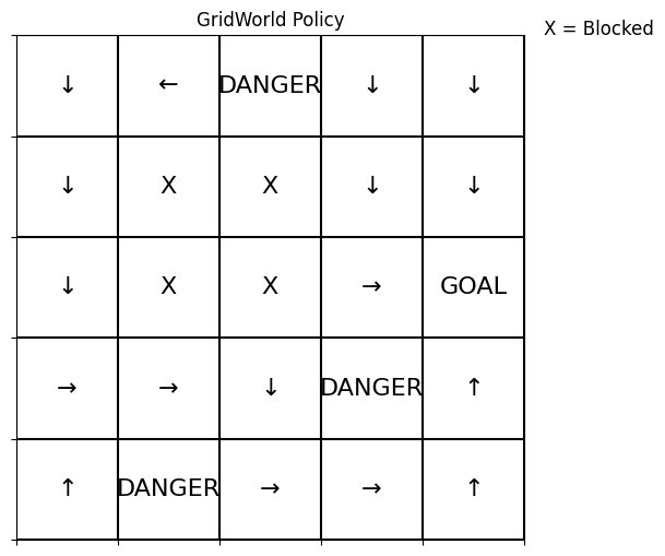
ii) with transition noise = 0.2

Again, we see that with noise, the algorithm still deduces a policy that allows you to reach the goal state from any starting state. The policy does not have a local maximum that prevents you from reaching the global maximum (goal state). The policy with noise is the same as the one deduced without noise, with the exception of the top right corner, where slightly different moves are picked. Since these moves result in the exact same end state as the policy with no noise, it is not very significant.
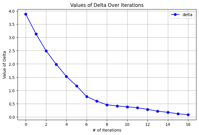
In this case we can see that the algorithm goes through more iterations, 17 to be exact, and the delta converges in a slower fashion. This is most likely caused by the noise which makes the transition function probabilistic and leads to more fluctuation and maybe more non-stationary values. This is also evident in the fact that the algorithm ends only because delta dropped below the threshold and is only approaching 0, not equal to 0 as was the case previously. This is evidence that increase in noise is a major factor in increasing convergence time and convergence path.
Since the policy is optimal and the delta converges (although it does not reach 0), the algorithm still performed quite well.