
distributed training with mlx: tensor parallelism
The content of this document was orginally intended to be merged into the MLX official docs as an example for tensor parallelism. It is currently in PR review here. Since I was proud of the effort and explanation I gave, I decided to cross post it here as well.
Tensor Parallelism in MLX
MLX enables efficient implementation of tensor parallelism (TP) through its implementation of distributed layers. In this example, we will explore what these layers are and create a small inference script for Llama family transformer models using MLX tensor parallelism.
Sharded Layers
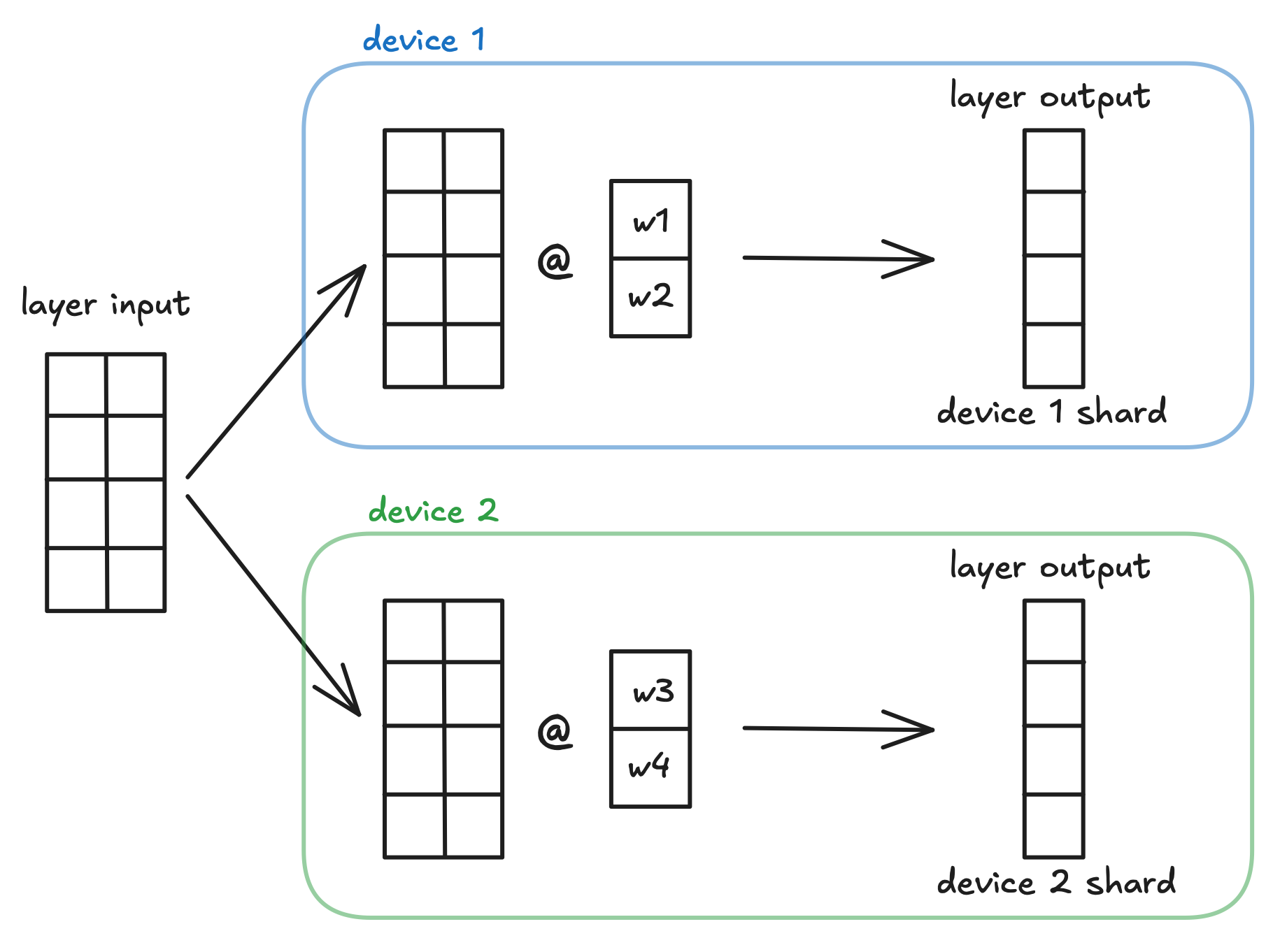
AllToShardedLinear
Column-wise tensor parallelism. This layer replicates a common input and shards the weight matrix along the output dimension (column-wise) across all devices in the mlx.core.distributed.Group. The layer produces a sharded output.
For example, consider an mlx.nn.AllToShardedLinear layer with input_dims=2 and output_dims=2, a batched input of shape (4, 2), and a device group with 2 devices. The layer shards the weight matrix column-wise across the two devices, where each device receives the full input and computes a partial output.
Check out huggingface ultrascale-playbook to learn more about tensor parallelism in LLMs.
This layer does not automatically gather all outputs from each device. This is an intended and useful design choice.
QuantizedAllToShardedLinear is the quantized equivalent of mlx.nn.AllToShardedLinear.
Similar to mlx.nn.QuantizedLinear, its parameters are frozen and
will not be included in any gradient computation.
ShardedToAllLinear
Row-wise tensor parallelism. This layer expects inputs that are sharded along the feature dimension (column-wise) and shards the weight matrix along the input dimension (row-wise) across all devices in the mlx.core.distributed.Group. The layer automatically aggregates the results using mlx.core.distributed.all_sum, so all devices in the group will have the same result.
For example, consider an mlx.nn.ShardedToAllLinear layer with input_dims=2 and output_dims=2, a batched input of shape (4, 2), and a device group with 2 devices. The layer shards the weight matrix row-wise and the input column-wise across the two devices. Each device computes a (4,2) output, which is then aggregated with all other device outputs to get layer output.
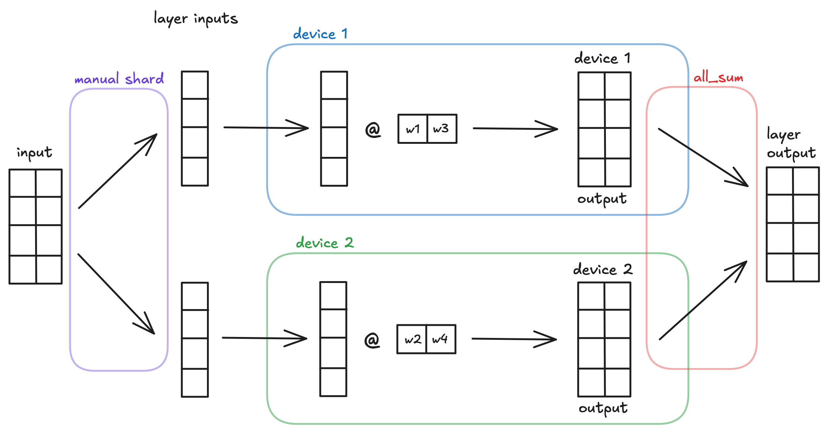
This layer does not automatically shard the inputs along the feature dimension for you. It is necessary to create a "partial" input structure to feed into the layer. This is an intended and useful design choice.
We can create partial inputs based on rank. For example, for an input with 1024 features, we can create sharded inputs in the following manner:
pythonworld = mx.distributed.init()
part = (
    slice(None), # batch dimension: keep all batches per feature
    slice(
        world.rank() * 1024 // world.size(), # start
        (world.rank() + 1) * 1024 // world.size(), # end
    ),
)

layer = nn.ShardedToAllLinear(1024, 1024, bias=False) # initialize the layer
y = layer(x[part]) # process sharded input
This code splits the 1024 input features into world.size() different groups which are assigned continuously based on world.rank(). More information about distributed communication can be found in the MLX distributed communication documentation.
QuantizedShardedToAllLinear is the quantized equivalent of mlx.nn.ShardedToAllLinear.
Similar to mlx.nn.QuantizedLinear, its parameters are frozen and
will not be included in any gradient computation.
Shard Utility Functions
shard_linear
Converts a regular linear layer into a tensor parallel layer that distributes computation across multiple devices. Takes an existing mlx.nn.Linear or mlx.nn.QuantizedLinear layer and returns a new distributed layer (either mlx.nn.AllToShardedLinear or mlx.nn.ShardedToAllLinear, depending on the sharding type). The original layer is not modified.
shard_inplace
Splits the parameters of an existing layer across multiple devices by modifying the layer in-place. Unlike shard_linear, this function does not create a new layer or add distributed communication. The layer itself must handle distributed communication if needed.
Useful Design Choices
The design choices above regarding when operations are done automatically are intentional and make model training and inference easier.
Column-wise and row-wise tensor parallel layers naturally go together because the output of the column-wise TP layer is exactly the size needed for the sharded input of a row-wise TP layer. This removes the need for an intermediate gather step between the layers, reducing communication overhead.
This is why AllToShardedLinear does not aggregate results automatically and why ShardedToAllLinear does not shard inputs automatically. It is so that they can be placed in successive order and work together easily.
We can demonstrate this through a simple model using our two types of distributed layers.
pythonx = ... # some (4, 2) model input: batch size 4, feature size 2

l1 = nn.AllToShardedLinear(2, 2, bias=False)   # initialize the layer
l1_out = l1(x) # (4, 1) output

l2 = nn.ShardedToAllLinear(2, 2, bias=False)
l2_out = l2(l1_out) # (4, 2) output
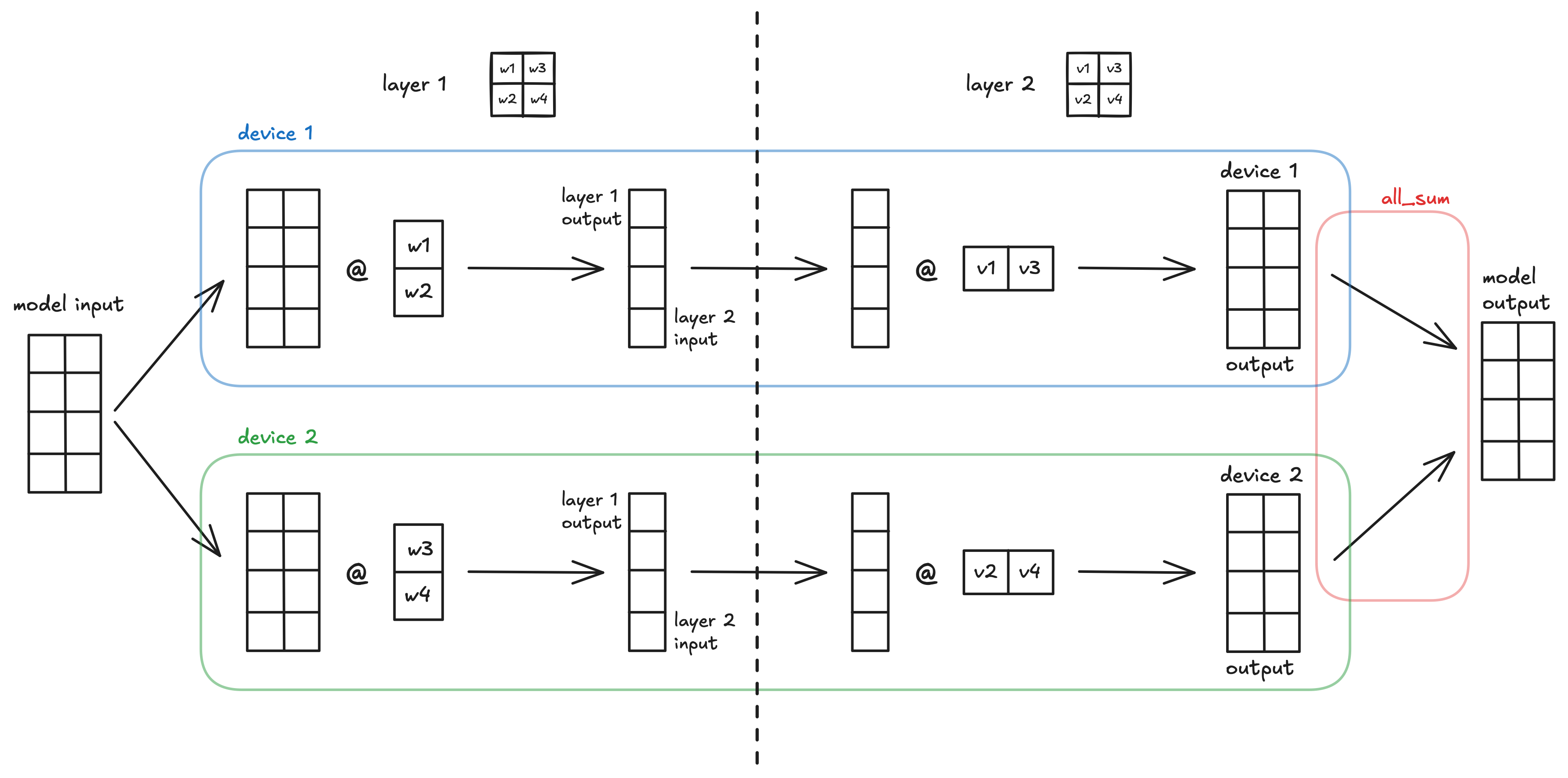
A visualization of the simple MLX model using column-wise then row-wise tensor parallelism across 2 devices.
LLM Inference with Tensor Parallelism
We can apply these TP techniques to LLMs in order to enable inference for much larger models by sharding parameters from huge layers across multiple devices.
To demonstrate this, let's apply TP to the Transformer block of a Llama Inference example. In this example, we will use the same inference script as the Llama Inference example, which can be found in mlx-examples.
Our first edit is to initialize the distributed communication group and get the current process rank:
pythonworld = mx.distributed.init()
rank = world.rank()
Next, let's look at the current architecture of the transformer block and see how we can apply tensor parallelism:
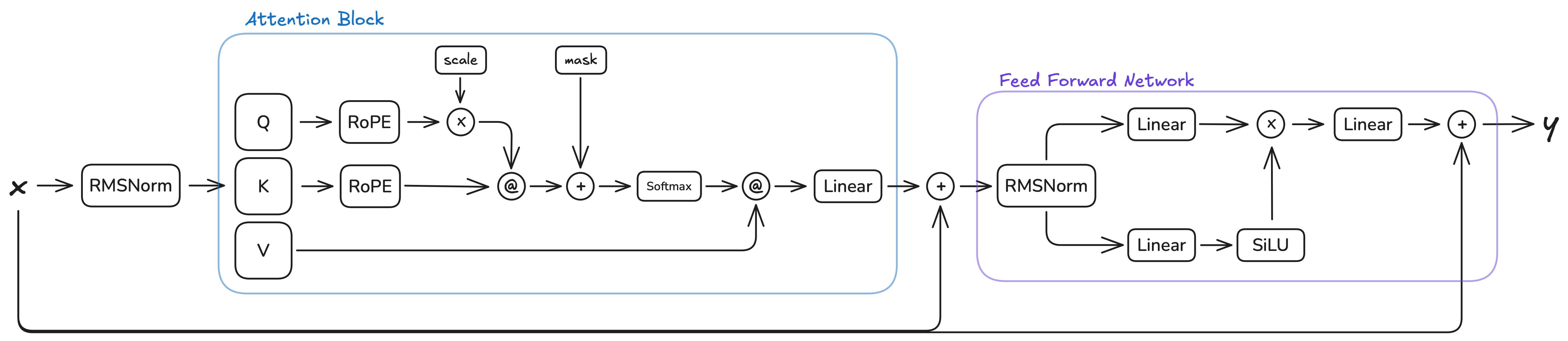
This architecture has two natural places where our column-wise then row-wise tensor parallelism paradigm can be applied: the attention block and the FFN block. Both follow the same pattern: multiple parallel linear layers operating on the same input, followed by a single output linear layer. In the attention block, the Q, K, and V projections are sharded column-wise, and the output projection is sharded row-wise. In the FFN block, the gate and up projections are sharded column-wise, and the down projection is sharded row-wise.
The intermediate operations between the linear layers (RoPE, softmax, scaled dot-product attention in the attention block, and element-wise multiplication in the FFN block) do not impede the use of our TP paradigm. These operations are either:
-
Element-wise operations (RoPE, element-wise multiplication): These operate independently on each element or position, preserving the sharding pattern without requiring cross-device communication.
-
Operations on non-sharded dimensions (softmax, scaled dot-product attention): These operate along dimensions that are not sharded (such as the sequence length or head dimensions), so they can be computed independently on each device. The attention computation
Q @ K^Tandscores @ Vwork correctly with sharded Q, K, V tensors because the matrix multiplications are performed along the sharded feature dimension, and the results remain properly sharded for the subsequent row-wise TP layer.
To implement sharding in our Llama inference, we use shard_linear to get sharded linear layers with distributed communication. This is easier than using shard_inplace and implementing the steps manually in the __call__ function.
The following code shows how to shard the Attention block. The Q, K, and V projection layers are converted to column-wise sharded layers (all-to-sharded), while the output projection is converted to a row-wise sharded layer (sharded-to-all). The number of heads and repeats are also adjusted to account for the sharding:
python# ... in Attention class
def shard(self, group: mx.distributed.Group):
  self.n_heads = self.n_heads // group.size()
  self.n_kv_heads = self.n_kv_heads // group.size()
  self.repeats = self.n_heads // self.n_kv_heads

  self.wq = nn.layers.distributed.shard_linear(self.wq, "all-to-sharded", group=group)
  self.wk = nn.layers.distributed.shard_linear(self.wk, "all-to-sharded", group=group)
  self.wv = nn.layers.distributed.shard_linear(self.wv, "all-to-sharded", group=group)
  self.wo = nn.layers.distributed.shard_linear(self.wo, "sharded-to-all", group=group)
Similarly, the FeedForward block is sharded by converting the gate (w1) and up (w3) projections to column-wise sharded layers, and the down projection (w2) to a row-wise sharded layer:
python# ... in FeedForward class
def shard(self, group: mx.distributed.Group):
  self.w1 = nn.layers.distributed.shard_linear(self.w1, "all-to-sharded", group=group)
  self.w2 = nn.layers.distributed.shard_linear(self.w2, "sharded-to-all", group=group)
  self.w3 = nn.layers.distributed.shard_linear(self.w3, "all-to-sharded", group=group)
Finally, in our load_model function, we need to apply our sharding functions to all transformer layers when using multiple devices:
python# ... in load_model function
if world.size() > 1:
  # convert Linear layers in Transformer/FFN to appropriate Sharded Layers
  for layer in model.layers:
      layer.attention.shard(group=world)
      layer.feed_forward.shard(group=world)
This allows us to use the llama inference file as normal when running python llama.py, but now we can also run it across two (or more) devices via mlx.launch -n 2 llama.py.
The entire runnable TP Llama inference script can be found in this PR