distributed training with mlx: data parallelism

Trying to profile how using distributed training techniques can improve the performance of LLM training on mac silicon devices.

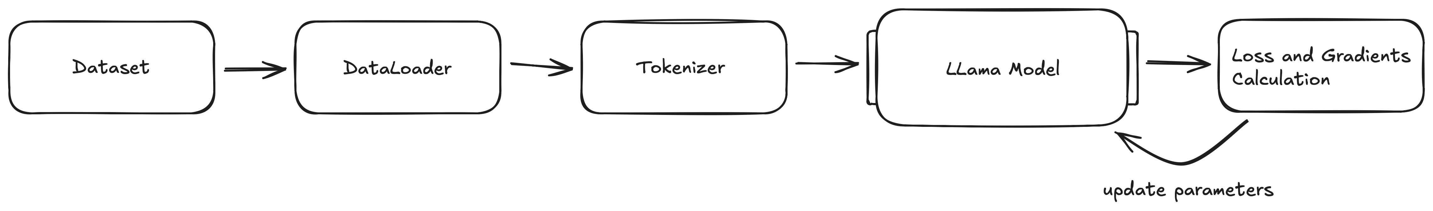
We first create the LLM architecture, by using MLX's LLama implementation found here. This saves us a lot of time. Next we generate a training harness that will take data from a dataset we proved, splitting the data into batches, tokenizing them, feeding them into our LLama model, calculating loss and gradient values and updating the model's parameters accordingly.

For the purpose of this investigation I am using the TinyStories dataset and huggingface's gpt2 AutoTokenizer.

Naive Training Implementation

The training file is simple and currently only contains the essentials. First, some configuration.

python
# Constants

BATCH_SIZE = 4
BLOCK_SIZE = 512
LEARNING_RATE = 3e-4
NUM_EPOCHS = 1
SEED = 42  

# Model Configuration (Small model)
MODEL_ARGS = {
	"num_layers": 4,
	"vocab_size": 50257, # GPT-2 vocab size
	"dims": 256,
	"mlp_dims": 512,
	"num_heads": 4,
}

            

a function to load the dataset and a function to iterate over the dataset to create batches:

python
def load_data_and_tokenizer():
	dataset = load_dataset("roneneldan/TinyStories", split="train", streaming=False)
	tokenizer = AutoTokenizer.from_pretrained("gpt2")
	tokenizer.pad_token = tokenizer.eos_token
	return dataset, tokenizer
	
def batch_iterate(dataset, tokenizer, batch_size, block_size):
	batch = []
	for example in dataset:
		text = example["text"]
		tokens = tokenizer.encode(text)
	
	# truncate or pad to block_size.
	if len(tokens) > block_size:
		tokens = tokens[:block_size]
	else:
		# Pad with eos_token
		tokens = tokens + [tokenizer.eos_token_id] * (block_size - len(tokens))
	batch.append(tokens)
	
	if len(batch) == batch_size:
		yield mx.array(batch)
	batch = []

            

There functions together form our primitive DataLoader. As we progress it will be important to progress on this design in order to make it easier to do load data and different batches across multiple processes or devices. I am also using the dataset from huggingface with streaming explicitly turned off. While streaming is a good feature for training and downloading data simultaneously (to save storage space and time), it becomes tedious to work with while testing. This is due to a significant latency between starting training and waiting for the first sequences to download and be compiled into a batch. I preferred to download the entire dataset once, and have faster startup times after.

Finally, we have the main() function which deals with the orchestrating of training. There are a couple parts to this function.

First there is the preparation steps:

python
mx.random.seed(SEED) # setting a seed to ensure reproducability of benchmarks
dataset, tokenizer = load_data_and_tokenizer() # load dataset and tokenizer
model = Model(**MODEL_ARGS) # create the model
mx.eval(model.parameters())
optimizer = optim.AdamW(learning_rate=LEARNING_RATE) # initialize optimizer

            

mx.eval() is special and deserves a bit more than a one line comment. MLX is lazy, so computations like c = a + b are not computed until they are explicitly told to do so. This allows for better optimization down the road by fusing operations together, but that is not super important at this moment. We just need to know that this needs to be called to compute actual values for the model parameters instead of their values just being pointers to other values.

Then we define a loss function, which computes the logits (outputs) of the model and uses cross entropy + mean to compute a loss value.

python
def loss_fn(x, y):
	logits = model(x)
	return nn.losses.cross_entropy(logits, y).mean()

            

Next, we create the step() function, which defines what we will do with each batch of training tokens.

python
def step(model, x, y):
	loss, grads = nn.value_and_grad(model, loss_fn)(x,y)
	optimizer.update(model, grads)
	return loss

            

Finally, we have our training loop, which we will limit to 100 batches since we are just testing. As we implement more and see promising results, this size will go up.

python
for batch in data_iter:
	inputs = batch[:, :-1]
	targets = batch[:, 1:]

	loss = step(model, inputs, targets)
	mx.eval(loss, model.parameters())
	
	step_count += 1
	
	print(f"Step {step_count}: Loss = {loss.item():.4f}")
	
	if step_count >= 100:
		break

            

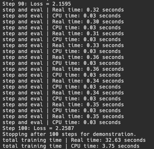
Now if we run this file, and we add some simple time profiling using python's built in time module, we can test the time it takes for each batch to execute, and how long it takes for all 100 batches to finish.

Ok, so now we have somewhat of a working training loop for an LLM. The first thing we can try is the simplest method of parallelism which is data parallelism.

Data Parallelism (DP)

initializing distributed communication and data parallelism (sorta)

Since I do not have a multiple mac setup at the moment, I can simulate multiple devices through multiple processes using mlx.launch utility. This will not give us good performance, but at least it will show if two processes can communicate and train properly.

In order to try this out, we need to understand data parallelism and then make the appropriate changes to our training code.

On GPUs (using only DP), each GPU would have a copy of the model in memory and would run a separate "micro-batch" of inputs through the model. Once all micro-batches have gone through the forward and backward pass of the model, the all-reduce communication primitive is used to assemble all the calculated gradients in order to optimize.

On Macs, we can do the exact same thing; we can load the model into the unified memory of each Mac, and run different micro-batches on each device and then compile all the gradients calculated to do one update step.

My first implementation of this will just be to take the existing batch loaded from the dataset and split it into two (across two processes). To do so using MLX, we must initialize the distributed environment inside of our training file.

python
world = mx.distributed.init()
rank = world.rank()
world_size = world.size()

            

world holds an object of type Group which represents the "world" of processes that can communicate. It holds the size of the Group and the specific rank that a process is inside of that group. The rank is a unique identifier of a process (or later a device) in the Group.

Additionally, we need to update our step function to accumulate gradients from all processes and consolidate them into one update vector for optimization. We can use MLX's built in utility average_gradients to do so.

python
def step(model, x, y):
	loss, grads = nn.value_and_grad(model, loss_fn)(model, x, y)
	grads = nn.average_gradients(grads) # sync step
	optimizer.update(model, grads)
	return loss

            

Next, we can implement a super simple batch splitting method to test if our distributed environment testing works (and I will explain why it is not truly DP yet later). We can keep the training loop code very similar to before and just change the way we assign inputs and targets to the following

python
for batch in data_iter:
	if (rank == 0):
		inputs = batch[0:2, :-1]
		targets = batch[0:2, 1:]
	elif (rank == 1):
		inputs = batch[2:, :-1]
		targets = batch[2:, 1:]

	# ... rest of training code ...

            

For each batch, I have hard coded a split of the batch of 4 into two batches of 2 inputs, and based on the rank of the process, it will either get the first 2 inputs or the last 2 inputs to form a micro-batch. I also made the print statements only happen if the process is rank 0, so that there wouldn't be multiple repeating statements. Then, we can run it using mlx.launch -n 2 dp_train.py and see the following

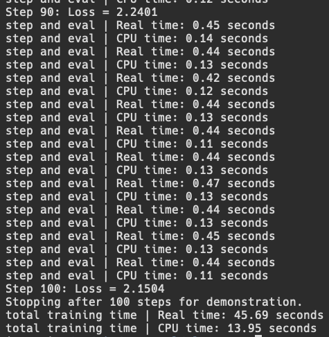
We can see that it works, but step and overall performance is worse, but this is likely because we are not optimizing correctly for multiple processes on the same device and losing time on added communication. It is difficult to find information about how multiprocessing happens through mlx.launch, but I hope to find out in the future through deeper research. Additionally, the main goal of DP is not to speed up such small batch sizes, but rather to allow for much much larger global batch sizes (split into micro batches across many devices) to exist and run efficiently. We will get there eventually.

I said before we ran this that this isn't exactly data parallelism and now I will explain why. Although we do have two separate processes computing forward and backward passes on separate micro batches, we are not actually reaping the benefits of DP. This is because each processes repeat each other.

Both processes use load_data_and_tokenizer and batch_iterate on the entire dataset, redoing the work that the other has done. This results in the dataset and all batches being loaded into memory twice and although the process is only processing half the batch, it has still loaded the entire batch. We can attempt to prove this is happening by using mlx.core.get_peak_memory() and/or mlx.core.get_active_memory().

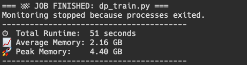
Our naive training implementation gives us a peak memory usage of around 2.17 GB, while our new DP training implementation gives us a peak memory usage of around 1.4 GB for each process. For better memory profiling, I asked Gemini to write me a bash script that constantly polls the dp_train.py processes for their memory consumption, which includes mlx.launch instance and two python instances of dp_train.py (can be read in depth in the repo).

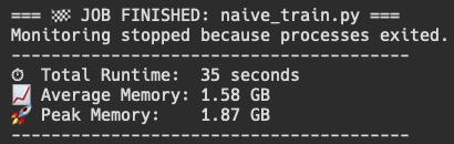
This gives us a way better idea of what is going on when we run a mlx.launch command to spawn 2 different processes, and also gives a baseline to improve on. Although results vary between runs (peak and average), it is definitely evident that "DP training" is using about double the memory of our naive training.

This proves that we have not actually implemented data parallelism yet and are currently wasting memory. It also does tell me that I would like to have more useful memory profiling tools for MLX on mac silicon. If anyone has suggestions lmk.

so... let's implement data parallelism (real)

How do we implement it the right way? We make sure to load only the data the process requires into memory. This is usually done by a dedicated Distributed Data Loader class which I plan on making in the future for this project, but until then we can explore this concept in a simpler way. A requirement that can mark our success in this journey is being able to spawn as many processes as we want and see little difference in the amount of memory used. This would mean that our dataset is only loaded once and all the processes are simply accessing or are sent the data they need.

Our problem lies mainly within the load_data_and_tokenizer function we implemented. Specifically,

python
dataset = load_dataset("roneneldan/TinyStories", split="train", streaming=False)

            

This line is using the load_dataset function from the datasets pip package from HuggingFace. Currently, every process that we spawn will run this line of code as a part of it initialization step. This effectively loads the entire dataset (or some part of the dataset) into memory for every process, causing much redundancy.

We can improve this by using the split feature on the load_dataset function and making it pull a different part of the dataset in order to only load everything once overall. We could also use the mlx.core.distributed.send functionality to send individual micro batches to each device/process, but we will explore that later and compare the differences. Here, by doing it this way we eliminate the communication step of sending batches to each process, but if we were using multiple devices, we would need a copy of the dataset on each one.

We can update the load_dataset implementation to the following,

python
shard_percentage = (100 / world_size)
shard_start = int(shard_percentage * rank)
shard_end = int(shard_start + shard_percentage)
dataset = load_dataset("roneneldan/TinyStories", split=f"train[{shard_start}%:{shard_end}%]", streaming=False)

            

This now uses a specified string format to load only a certain percentage in the data, based on the rank of the process and size of the world. In our test case with 2 processes, rank 0 will load 0% to 50% of the training dataset and rank 1 will load 50% to 100%. If we run this now, we should see that our memory consumption has gone down to almost match the memory consumption of running our naive training.

We can also use a more robust method to get equal sized splits described in the HF Loading documentation which is to use pct1_dropremainder. This may eliminate some examples in the dataset if they don't divide evenly among the processes/devices, but will make the future easier for us in terms of synchronization. This can be done by changing the split argument to:

python
split=f"train[{shard_start}%:{shard_end}%](pct1_dropremainder)"

            

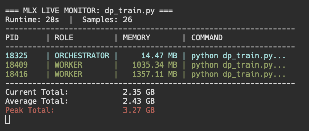
While running, we can notice some interesting things. First, one process is somehow using less memory than the other process. Second, the peak memory usage is still quite high at 3.27 GB. Third, our average total is quite low!

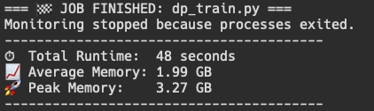
After the entire run finished, we can now see that the average memory usage of the DP training file is much reduced, and only around 300 MB larger than the naive training implementation. While 14.47 MB are being used by the orchestrator, there are many other things that could be contributing to this increase, but at least we are now not loading the entire dataset twice.

In the future I will build a much more robust data loader as a class to allow for many different datasets to be loaded and to also get a chance to see this running on two separate devices with varying amount of available memory.