distributed model training and DeMo

Nous Research's exploration into latency reduction during the training of large language models across limited bandwidth connections and heterogenous hardware. This is accomplished through the introduction of a new optimizer "DeMo: Decoupled Momentum Optimization" to replace AdamW, the current most popular deep learning optimizer.

Since current language models require very high parameter counts (billions), it is required to have multiple accelerators (GPUs, TPUs, etc.) in order to distribute the workload and achieve reasonable training times.

There are two main ways of achieving the distribution of model training to multiple accelerators: Distributed Data Parallelism and Fully Sharded Data Parallelism.

Distributed Data Parallelism: splitting up the data and training each section of the data independently?

Full Sharded Data Parallelism: splitting up the model parameters and having different machines train different "shards" of parameters?

In either scenario, both distributed techniques require the intensive process of synchronizing gradients in order to compute the optimizer step and update parameters. With an optimizer such as AdamW, the volume of communication needed for this synchronization step is often just as big as the model itself. This requires extremely high speed interconnections between the accelerators, which is only possible in localized networks. This means all the accelerators must be present together in some data center.

DeMo aims to significantly reduce the amount of data needed to be communicated in this synchronization step without sacrificing optimization results, thereby significantly reducing the latency of inter-network/non-localized distributed training. This is done by exploiting optimizer state redundancy, allowing the states to be highly compressed.

relevant background

The paper mentions three current approaches which aim to reduce communication overhead in distributed training.

Quantization and Sparsification of Gradients: Quantization works in the same way as it would in any other compression algorithm (e.g. JPEG). Say a gradient is represented as a 16-bit floating point number. You can chop the least significant bits off to reduce its size in memory, while losing precision. The limit to this is obviously the fact that you cannot go below 1-bit (but a 1-bit gradient doesn't seem very useful). Sparsification works by dropping data points in the gradient vectors and then appropriately amplifying the remaining data points in the vector to ensure no bias is introduced. This technique is theoretically unbounded, but again with high compression comes degraded training performance.

Low Rank Projection: LLM gradients have been shown to exhibit low rank structure. This means the the matrices defined by gradients during training generally represent low-dimensional vector spaces (defined by the number of linearly independent columns of said matrix). This enables the use of Singular Value Decomposition (SVD), which is essentially the process of projecting gradients onto lower-dimensional spaces, while still maintaining the major directions of the original gradient. This still is a bottleneck as you increase model size as SVD/projection computations provide significant compute overhead.

Federated Averaging: This method allows for nodes to train independently for multiple passes of the three step process of DNNs (forward pass, backward pass and optimization calculation) before synchronizing through weight averaging. Since this is not compressing the synchronized data, it still requires the same amount of bandwidth, but eliminates the need for per-step communication. There is also a trade off: more steps between synchronization leads to faster iterations, but poorer convergence. Finding the perfect balancing point between convergence quality and iteration speed is tough, and not suitable for a general purpose solution.

The paper also mentions that there are more communication optimization techniques which are clock-asynchronous or decentralized, but because of their complexity and very specific use cases, they were not mentioned.

methodology

The DeMo optimizer is built on three assumptions, conjectures without proof which are just based on findings of previous LLM training the Nous Research team has conducted.

To understand these conjectures, we must understand what they are based on: stochastic gradient descent.

stochastic gradient descent and momentum

Stochastic Gradient Descent (SGD) is a process of using stochastic approximation to speed up the calculations of normal gradient descent while keeping relatively accurate convergence. In traditional gradient descent, the gradient of a specific data vector in the multi dimensional space of the objective function (the function you are trying to minimize) is calculated using the entire dataset. Instead, with stochastic approximation, an estimate of the gradient is formed through a randomly selected subset of the data. This makes iterations in training much faster, but, again, has a trade off of a slower convergence rate. It also has the benefit of being able to navigate spaces with noisy data better, since gradient directions are less affected by outliers in the data when they are not calculated using all of the data points.

Momentum in SGD is a technique used to accelerate the optimization process and improve convergence. It does so by adding fractions of the previous optimization update to the current update. This speeds up convergence in direction with consistent gradient directions. So, essentially, as multiple gradients through out iterations show consistent movement in some directions, the sizes of the "steps" of the optimizer in that direction increases proportionally. This means the optimizer "gains momentum" in the prevalent gradient directions.

assumptions/conjectures

conjecture 1

"The fast-moving components of momentum exhibit high spatial auto-correlation, with most of their energy concentrated in a small number of principal components."

Interpretation: The "fast-moving" components of momentum are those directions of the gradient which are present across many iterations. They are said to exhibit "high spatial auto-correlation", which means that nearby points (in the space) have similar values to the fast-moving components. The second half the statement suggests that these components are concentrated in a few dominant directions, so dimensionality reduction techniques can be used to extract the few directions that capture most of their behaviour.

conjecture 2

"Fast-moving momentum components show low temporal variance and should be applied to parameter updates immediately, while slow-moving components exhibit high temporal variance and benefit from temporal smoothing over longer periods."

Interpretation: Fast-moving components have low variability over time, which implies they change consistently and predictably. These components should be applied to parameter updates immediately because they do not introduce noise or slow convergence. Slow-moving components have high variability over time, and therefore benefit from "temporal smoothing" such as exponential moving averages to stabilize their contribution to the optimization algorithm.

conjecture 3

"Slow-moving momentum components, despite their high variance, are crucial for long-term convergence and should be preserved rather than filtered out."

Interpretation: Although slow-moving components show high variability and introduce noise, they should still not be filtered out because they are very important for long-term convergence. Although they may initially seem noisy, they may represent larger-scale trends or adjustments that take longer to stabilize, but are just as important as the fast-moving components.

algorithm

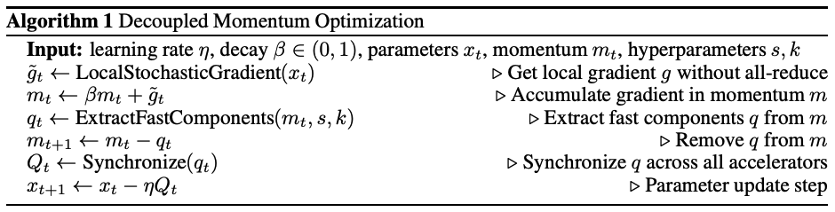
The algorithm is SGD with Momentum, but changed slightly (eh, more like a lot). First the local SGD is calculated on each processing unit (accelerator, whatever you want to call it). Then, the gradients from the current step (and previous momentum value m) are used to calculate the new momentum vector m. With this momentum vector, an algorithm is used to extract the fast moving components and then the fast moving components are removed from the momentum vector. Now an all-gather can be used to only synchronize the fast moving components q. From there the synchronized data can be used to calculate the parameter update using descent with a hyperparameter learning rate.

The algorithm above is reliant on an algorithm that can extract fast components efficiently. Based on Conjecture 1 it is possible to apply a spatial Kosmabi-Karhunen-Loeve Transform (KLT), which I will not explain because it will probably make this blog post 25 pages long (just kidding I am too lazy to read its wiki). Essentially the KLT helps them remove fast moving components based on their high spatial auto-correlation. Luckily for me as a reader of this paper, they do not use KLT, but rather a Discrete Cosine Transform (DCT) as an approximation of KLT. They are both "decorrelating" transforms, which are transforms that have the affect of reducing autocorrelation within a signal. Ok, that might not make the most sense, but let's just keep going because it will start too (hopefully). DCT is awesome, and widely used across tech (most notably in JPEG compression algorithms, shout out Mr.Stewart). Due to this, it has been made highly efficient on modern GPUs, and high parallelizable. Additionally, its complexity scales linearly with dimension increase and has a fixed basis, so you don't need to transfer any information over to decode a DCT encoded signal (everyone knows the basis). It's said to not be perfect, but this is perfect for a practical application of a super fast training algorithm.

Ok, so we want to use DCT to extract fast moving components. How is that achieved? Ok so to skip all the mathematical stuff (I don't want to type it all in LaTeX), basically, the momentum tensor from our second step of the algorithm is a d-dimensional auto-correlated signal that we chunk into d chunks. To each chunk we apply a DCT transform, that naturally has the property of decorrelating the chunk. DCT gives us back the coefficients of the basis functions of the cosine space and the waves with the highest coefficients are the most dominant frequencies in that chunk. We find the top-k (k is a hyperparameter) DCT coefficients in each chunk and store their frequencies (waves: cosine basis functions). These are our principal components of the momentum. At this point we have used DCT to effectively do a smarter low-rank projection and we have a set of frequencies that represent the principal components of the momentum.

The fast-moving principal components are then removed from the current momentum value, creating the momentum value to be used in the next step of the algorithm. This is seen in step 4 and is because we do not want to lose the slow-moving components of the momentum (according to conjecture 3). We can see that through synchronization we are applying the fast-moving components immediately and through step 4, we are letting the slow-moving components affect the gradient descent gradually (conjecture 2). The slow-moving components are "decoupled", hence the name of the optimizer. They change independently in each node, but they are effecting the fast-moving components coming out of each node over time, meaning they are gradually transmitted alongside the fast-moving components.

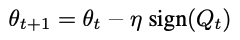
Finally, the optimizer may use a signum variant in order to improve convergence, but is optional.

experimental results

To train a model using DeMo, the OLMo framework was used. The Allen AI institute offers complete access to their models, training data and even the training code used. With some tweaks to the training code by including the DeMo (signum variant) optimizer class and disabling gradient synchronization in PyTorch Distributed Data Parallelism. The model was pre-trained on the Dolma v1.5 data. The model was trained on 100 billion total tokens rather than the full 3 trillion tokens in the Dolma training set.

The DeMo optimizer model was compared with the OLMo-1B model which was also trained on the 100 billion tokens (with adjusted learning rate schedule). The experiments were also repated on a smaller 300M model made by halving the OLMo-1B hidden size. All model training was performed on 64 H100 GPUS.

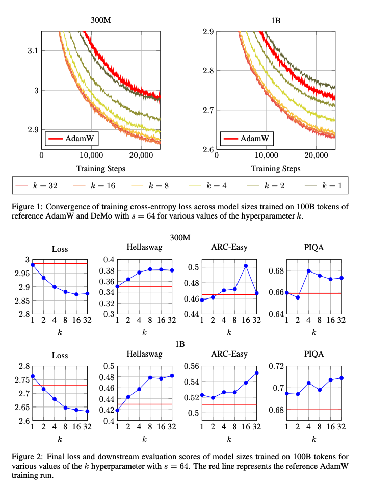
These were the results! The k values is the hyper parameter that decides the number of frequencies taken from each chunk in the DCT step.

From the figures, at the top, we can see that the DeMo optimizer allows for comparable convergence compared to AdamW. On the bottom we can see the performance of the models on test datasets, and the results are quite sporadic, but in either case, the scale on the y-axis indicates that the model trained with the DeMo optimizer normally performs just the same as one trained with AdamW.

food for thought

The OLMo-1B model was said to have been retrained with adjusted learning rates to compensate for the shorter schedule. I wonder if these hyperparameters were tweaked in such a way to make the DeMo optimizer look better than it is. This would need a lot of investigation into the supplementary code.

Furthermore, I wonder how a model with 3B or more parameters would converge with the DeMo optimizer and what the performance of such a model would be lie.

Anyway, I think this was a great paper and Nous Research is really pushing the boundaries of distributed model training. Maybe one day in the future I'll be able to train a LLM on my school labs computers (probably not).

references

[1] https://arxiv.org/pdf/2411.19870